Geometry
Introduction
We start with the simplest vocabulary of images, with “left” and “right” and “one, two, three,” and before we know how it happened the words and numbers have conspired to make a match with nature: we catch in them the pattern of mind and matter as one.
Imagine that you have control of a little creature called a turtle that exists in a mathematical plane or, better yet, on a computer display screen.
The turtle can respond to a few simple commands:
forwwardmoves the turtle, in the direction it is facing, some number of units.rightrotates it in place, clockwise, some number of degrees.backandleftcause the opposite movements.
The number that goes with a command to specify how much to move is called the command’s input.
In describing the effects of these operations, we say that:
forwardandbackchange the turtle’s position (the point on the plane where the turtle is located)rightandleftchange the turtle’s heading (the direction in which the turtle is facing).
The turtle can leave a trace of the places it has been: The position-changing commands can cause lines to appear on the screen. This is controlled by the commands penup and pendown. When the pen is down,
the turtle draws lines.
In describing the effects of these operations, we say that forward and back change the turtle’s position (the point on the plane where the turtle is located); right and left change the turtle’s heading (the direction in which the turtle is facing).
The turtle can leave a trace of the places it has been: The position-changing commands can cause lines to appear on the screen. This is controlled by the commands penup and pendown. When the pen is down, the turtle draws lines.
Function
Turtle geometry would be rather dull if it did not allow us to teach the turtle new functions.
But luckily all we have to do to teach the turtle a new trick is to give it a list of functions it already knows.
For example, here’s how to draw a square with sides 100 units long:
This is an example of function.
The first line of the funcion definition specifies the function’s name. We’ve chosen to
name this procedure square, but we could have named it anything at all.
The rest of the function (the body) specifies a list of instructions the turtle is to carry out in response to the square command.
There are a few useful tricks for writing functions. One of them is called iteration, meaning repetition doing something over and over.
Here’s a more concise way of telling the turtle to draw a square, using iteration:
This procedure will repeat the indented commands forward(100) and right(90) four times.
Another trick is to create a square procedure that takes an input for the size of the square.
To do this, specify a name for the input in the title line of the function, and use the name in the function body:
Now, when you use the command, you must specify the value to be used for the input, so you say square(100), just like forward(100).
The chunk forward(size) and right(90) might be useful in other contexts, which is a good reason to make it a function in its own right:
Now we can rewrite square using square_piece as
Notice that the input to square, also called size, is passed in turn as an input to square_piece.
square_piece can be used as a function in other places as well - for example, in drawing a rectangle:
To use the rectangle function you must specify its two inputs, for example, rectangle(100,50).
Drawing
Let’s draw a figure that doesn’t use 90ᵒ angles an equilateral triangle.
Since the triangle has 60° angles, a natural first guess at a triangle function is:
But triangle doesn’t work:
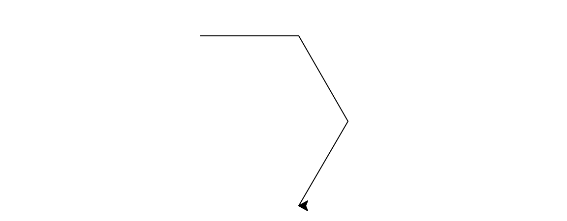
In fact, running this “triangle” function draws half of a regular hexagon.
The bug in the procedure is that, whereas we normally measure geometric figures by their interior angles, turtle turning corresponds to the exterior angle at the vertex.
So if we want to draw a triangle we should have the turtle turn 120°.
You might practice “playing turtle” on a few geometric figures until it becomes natural for you to think of measuring a vertex by how much the turtle must turn in drawing the vertex, rather than by the usual interior angle.
Turtle angle has many advantages over interior angle, as you will see.
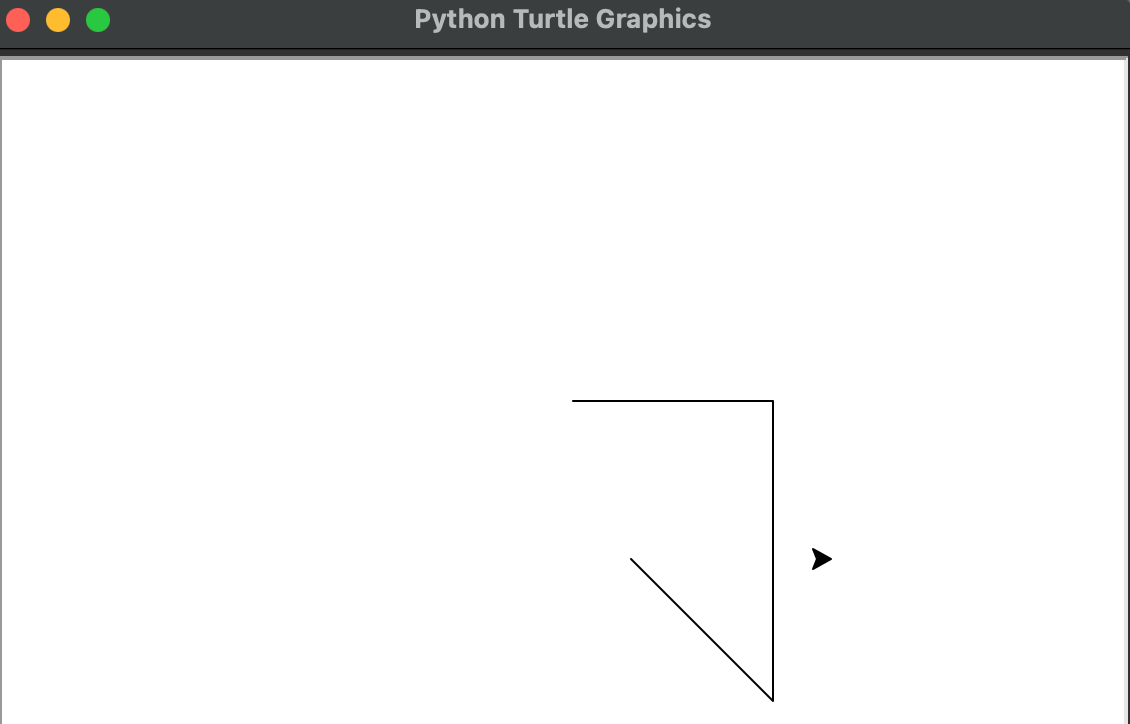
Now that we have a triangle and a square, we can use them as building blocks in more complex drawings – a house, for example.
But simply running square followed by triangle doesn’t quite work. The reason is that after square, the turtle is at neither the correct position nor the correct heading to begin drawing the roof.
To fix this bug, we must add steps to the procedure that will move and rotate the turtle before the triangle procedure is run.
In terms of designing programs to draw things, these extra steps serve as an interface between the part of the program that draws the walls of the house (the square function) and the part that draws the roof (the triangle function).
In general, thinking of functions as a number of main steps separated by interfaces is a useful strategy for planning complex drawings.
Using functions and functions that call functions is also a good way to create abstract designs.
This code shows how to create elaborate patterns by rotating a simple “doodle.”
Circle
After all these straight line drawings, it is natural to ask whether the turtle can also draw curves circles, for example.
One easy way to do this is to make the turtle go forward a little bit and then turn right a little bit, and repeat this over and over:
This draws a circular arc
Since this program goes on “forever” (until you press the stop button on your computer), it is not very useful as a subprocedure in creating more complex figures.
More useful would be a version of the circle procedure that would draw the figure once and then stop.
When we study the mathematics of turtle geometry, we’ll see that the turtle circle closes precisely when the turtle has turned through 360°.
So if we generate the circle in chunks of forward(1) and right(1), the circle will close after precisely 360 chunks:
If we repeat the basic chunk fewer than 360 times, we get circular arcs.
For instance, 180 repetitions give a semicircle, and 60 repetitions give a 60° arc.
The following procedures draw left and right arcs of deg degrees on a circle of size r:
The circle program above actually draws regular 36Ogons, of course, rather than “real” circles, but to make drawings on the display screen, this difference is irrelevant.
Turtle Geometry versus Coordinate Geometry
We can think of turtle commands as a way to draw geometric figures on a computer display.
But we can also regard them as a way to describe figures.
Let’s compare turtle descriptions with a more familiar system for representing geometric figures – the Cartesian coordinate system, in which points are specified by two numbers, the x and y coordinates relative to a pair of axes drawn in the plane.
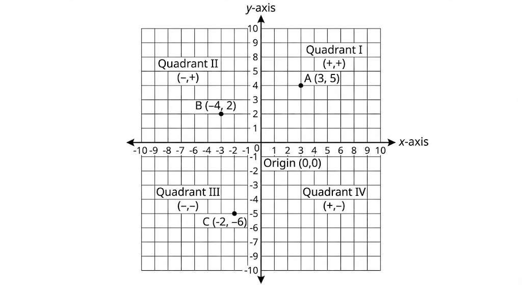
The turtle forward and right commands give an alternative way of measuring figures in the plane, a way that complements the
coordinate viewpoint.
The geometry of coordinates is called coordinate geometry; we shall refer to the geometry of forward and right as turtle geometry.
And even though we will be making use of coordinates later on, let us begin by studying turtle geometry as a system in its own right.
Whereas studying coordinate geometry leads to graphs and algebraic equations, turtle geometry will introduce some less familiar, but no less important, mathematical ideas.
Intrinsic versus Extrinsic
One major difference between turtle geometry and coordinate geometry rests on the notion of the intrinsic properties of geometric figures.
An intrinsic property is one which depends only on the figure in question, not on the figure’s relation to a frame of reference. The fact that a rectangle has four equal angles is intrinsic to the rectangle.
But the fact that a particular rectangle has two vertical sides is extrinsic, for an external reference frame is required to determine which direction is “vertical.”
Turtles prefer intrinsic descriptions of figures.
For example, the turtle program to draw a rectangle can draw the rectangle in any orientation (depending on the turtle’s initial heading), but a cartesian program would have to be modified if we did not want the sides of the rectangle drawn parallel to the coordinate axes, or one vertex at (0,0).
Another intrinsic property is illustrated by the turtle program for drawing a circle: Go forward a little bit, turn right a little bit, and repeat this over and over.
Contrast this with the Cartesian coordinate representation for a circle, x2 + y2 = r2.
The turtle representation makes it evident that the curve is everywhere the same, since the process that draws it does the same thing over and over. This property of the circle, however, is not at all evident from the Cartesian representation.
Compare the modified program
with the modified equation x2 + 2y2 = r2.
The drawing produced by the modified program is still everywhere the same, that is, a circle. In fact, it doesn’t matter what inputs we use to forward or right (as long as they are small). We still get a circle. T
The modified equation, however, no longer describes a circle, but rather an ellipse whose sides look different from its top and bottom.
A turtle drawing an ellipse would have to turn more per distance traveled to get around its “pointy” sides than to get around its flatter top and bottom. This notion of “how pointy something is,” expressed as the ratio of angle turned to distance traveled, is the intrinsic quantity that mathematicians call curvature.
Local versus Global
The turtle representation of a circle is not only more intrinsic than the Cartesian coordinate description.
It is also more local; that is, it deals with geometry a little piece at a time.
The turtle can forget about the rest of the plane when drawing a circle and deal only with the small part of the plane that surrounds its current position.
By contrast, x<sup>2</sup> + y<sup>2</sup> = r<sup>2</sup> relies on a large-scale, global coordinate system to define its properties.
And defining a circle to be the set of points equidistant from some fixed point is just as global as using x<sup>2</sup> + y<sup>2</sup> = r<sup>2</sup>. The turtle representation does not need to make reference to that “faraway” special point, the
center.
The fact that the turtle does its geometry by feeling a little locality of the world at a time allows turtle geometry to extend easily out of the plane to curved surfaces.
Functions versus Equations
A final important difference between turtle geometry and coordinate geometry is that turtle geometry characteristically describes geometric objects in terms of functions rather than in terms of equations.
In formulating turtle-geometric descriptions we have access to an entire range of procedural mechanisms (such as iteration) that are hard to capture in the traditional algebraic formalism.
Moreover, the procedural descriptions used in turtle geometry are readily modified in many ways.
Simple Turtle Programs
If we were setting out to explore coordinate geometry we might begin by examining the graphs of some simple algebraic equations.
Our investigation of turtle geometry begins instead by examining the geometric figures associated with simple procedures.
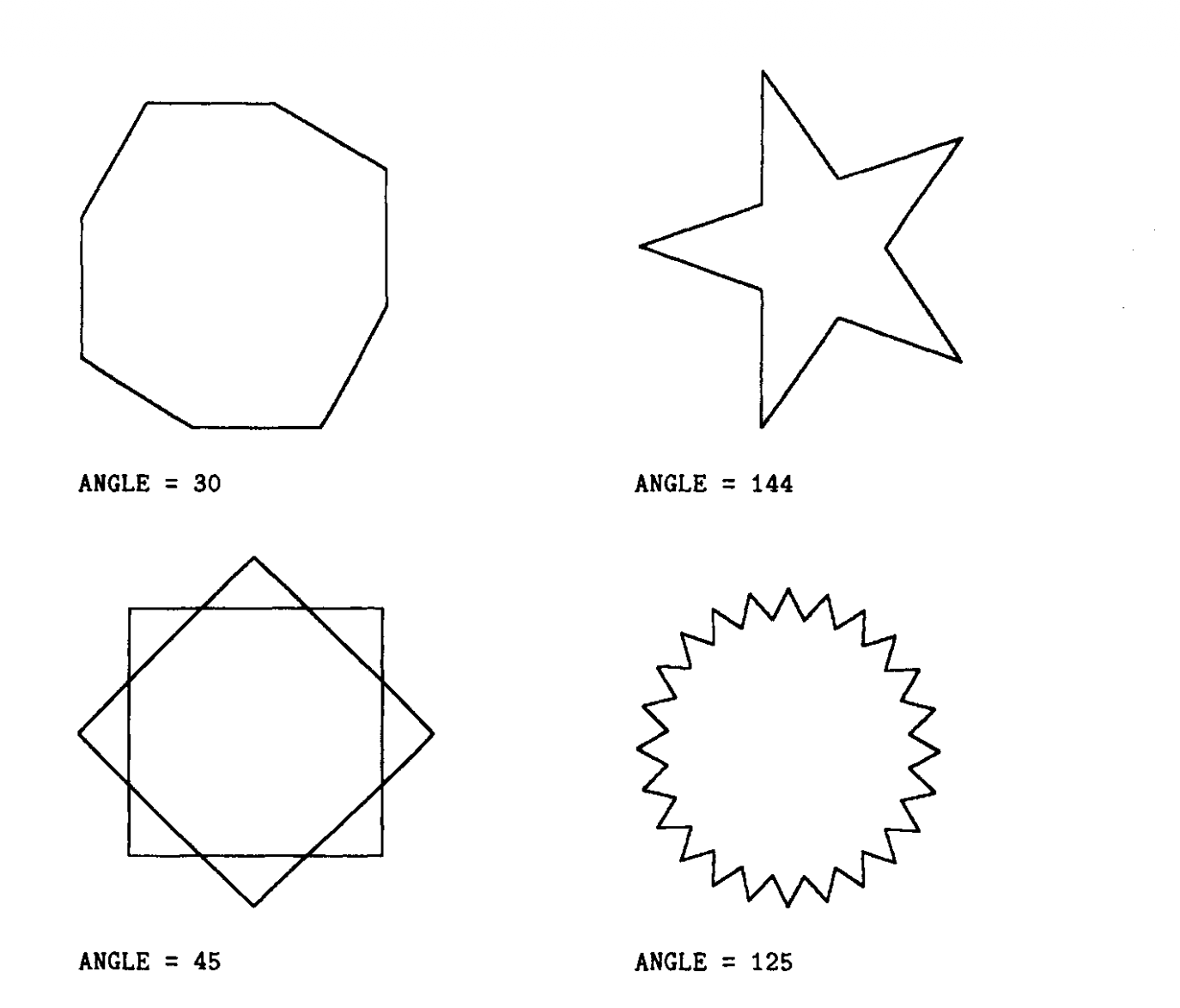
Here’s one of the simplest: Go forward some fixed amount, turn right some fixed amount, and
repeat this sequence over and over. This procedure is called poly.
It draws shapes like those:
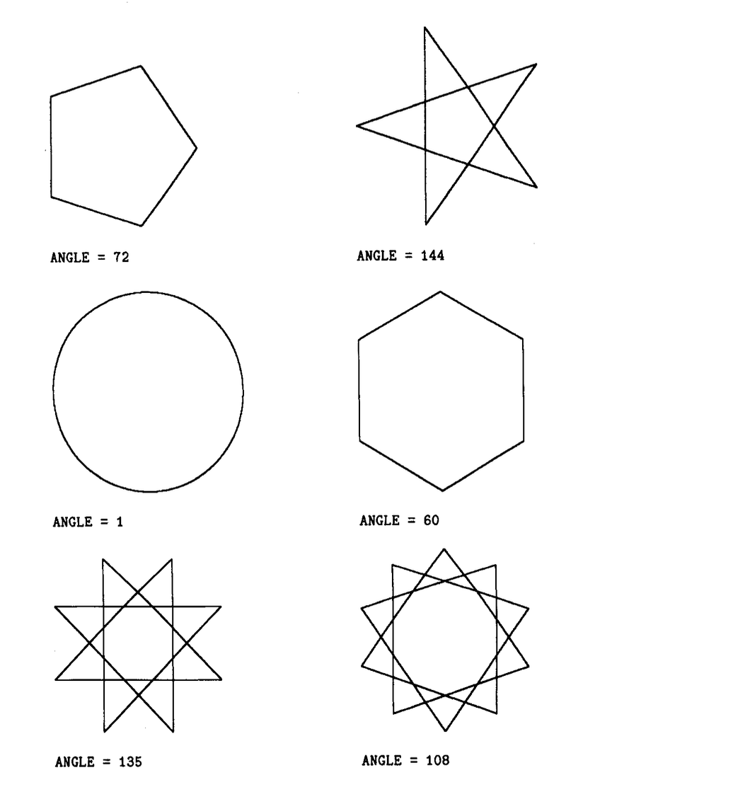
poly is a generalization of some procedures we’ve already seen:
- Setting the angle inputs equal to 90, 120, and 60, we get, respectively, squares, equilateral triangles, and regular hexagons.
- Setting the angle input equal to 1 gives a circle.
Spend some time exploring poly, examining how the figures vary as you change the inputs.
Observe that rather than drawing each figure only once, poly makes the turtle retrace the same path over
and over. (Later on we’ll worry about how to make a version of poly that draws a figure once and then stops.)
Another way to explore with poly is to modify not only the inputs, but also the program; for example
You should have no difficulty inventing many variations along these lines, particularly if you use such
functions as square and triangle as functions to replace or supplement forward and right.
Recursion
One particularly important way to make new procedures and vary old ones is to employ a program control structure called recursion; that is, to have a procedure use itself as a subprocedure, as in
The final line keeps the process going over and over by including “do poly again” as part of the definition of poly.
One advantage of this slightly different way of representing poly is that it suggests some further modifications to the basic program.
For instance, when it comes time to do poly again, call it with different inputs:
Follow there are some new sample poly figures:
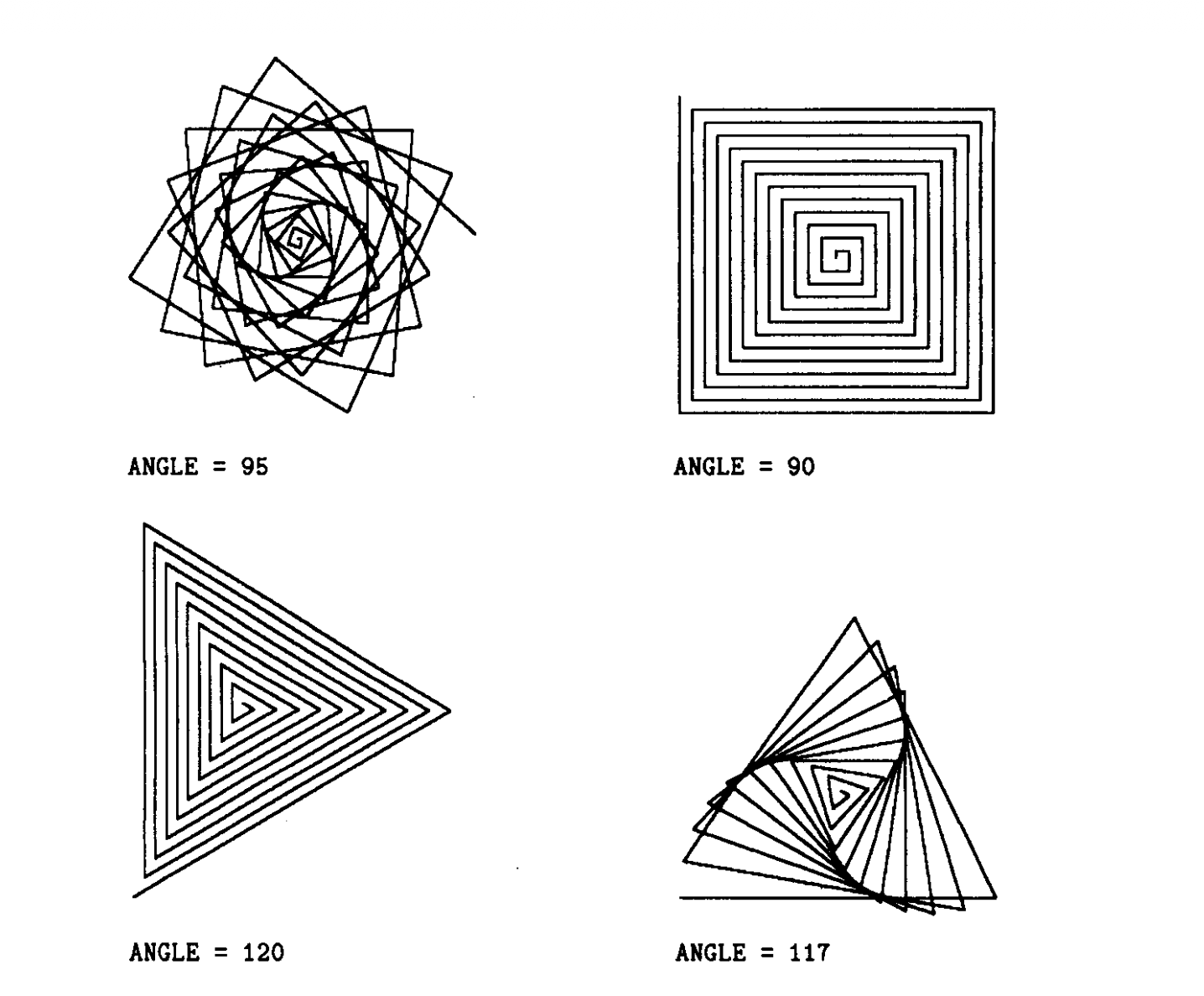
Look carefully at how the program generates these figures: Each time the turtle goes forward it goes one unit farther than the previous time.
A more general form of poly uses a third input (inc, for increment) to allow us to vary how quickly the sides grow:
In addition to trying poly with various inputs, make up some of your own variations:
- For example, subtract a bit from the side each time, which will produce an inward spiral.
- Or double the side each time, or divide it by two.
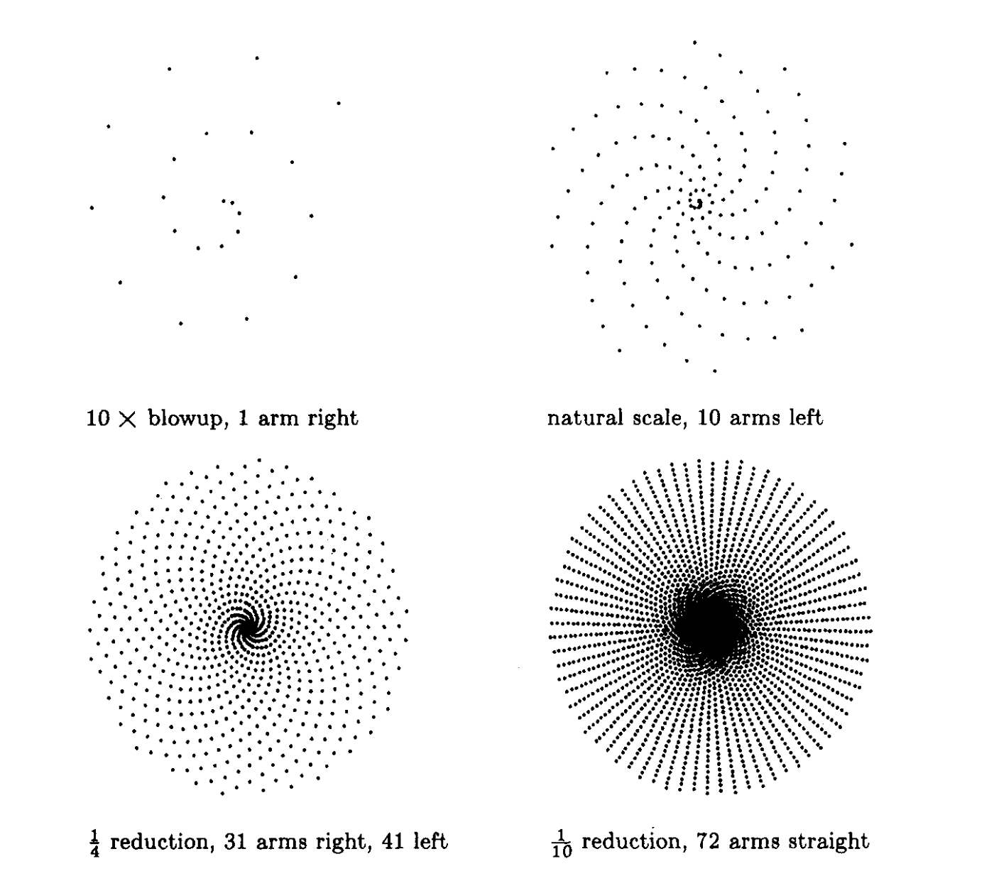
Figure illustrates a pattern made drawing only the vertices of poly, shown at four scales of magnification:
Another way to produce an inward spiral (curve of increasing curvature) is to increment the angle each time:
Run spiral and watch how it works.
The turtle begins spiraling inward as expected. But eventually the path begins to unwind as the angle is incremented past 180°.
Letting spiral continue, we find that it eventually produces a symmetrical closed figure which the turtle retraces over and over as shown in the next figure:

You should find this surprising.
Why should this succession of forwards and rights bring the turtle back precisely to its starting point, so that it will then retrace its own path?
We will see in the next section that this closing phenomenon reflects the elegant mathematics underlying turtle geometry.